Querying
For this we’re going to be using the same examples as can be found here. That is we have a database for a university, with four tables:
Schools - a university may have several schools, for example the school of science, the school of arts, and the school of business. The school table has the following columns:
- A code (primary key)
- A name
- A campus - north campus, south campus, etc.
Programs - each school may offer several programs, or degrees - a bachelor of commerse, a bachelor of arts, or a master of arts. The program title has the following columns:
- A code (primary key)
- A school code (foreign key)
- A title (e.g. bachelor of commerce)
- A degree type - bachelor’s, masters, phd, etc.
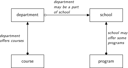
Departments - for example, the physics department might be a part of the school of science. Each department has:
- A code (primary key)
- A name
- A school code (foreign key)
Courses - Departments offer courses, this is pretty self explanatory. each course has
- A course code (primary key)
- A department code (foreign key)
- A number of credits
- A description
- A title
This is summarized in the following diagram:
The Query Object
Tables are set up in the “Examples” folder of the github repo located at https://github.com/xnmp/lambdaquery. The boilerplate code should be fairly self-explanatory and it’s worth glancing over it to see the syntax.
Use the Query.sql method to display the SQL of a query.
ex1 = School.query()
print(ex1.sql())
This will give the result:
SELECT DISTINCT
  sc_kda8.school_code AS code,
  sc_kda8.name AS name,
  sc_kda8.campus AS campus
FROM school AS sc_kda8
Filtering
Use the .filter method to filter:
School.query().filter(lambda x: x.campus == 'south')
Since this construction is so common, this can be abbreviated down to:
School.query(lambda x: x.campus == 'south')
The resulting SQL looks like:
SELECT DISTINCT
  sc_pob4.school_code AS code,
  sc_pob4.name AS name,
  sc_pob4.campus AS campus
FROM school AS sc_pob4
WHERE (sc_pob4.campus = 'south')
Selecting
To demonstrate selecting, we use the fmap method of the query object. Again, we can think of a query like a list, and the fmap method is like mapping a function over that list. Selection looks like:
School.query().fmap(lambda x: x.name % x.campus)
Here we can think of the query as a list of dictionaries where the entries of the dictionary can be accessed by using an attribute name. The % operator herre can be thought of the operator that combinbes two dictionaries.
Note that because this is so common, a simpler way to do this is via the getitem method as follows:
School.query()['name','campus']
This will give the result:
SELECT DISTINCT
  sc_pob4.name AS name,
  sc_pob4.campus AS campus
FROM school AS sc_pob4
Now there’s always several ways to do things in LambdaQuery, and its strength lies in using a generator function to “unroll” a query. We can do this via the yield keyword, so that when we write sc0 = yield School.query() this can be thought of as for sc0 in School.query():. Then sc0 is a single school, and we can apply functions that work on single schools to sc0, such as, say, the number of departments it has.
For reference, the above is written using the generator function as:
@do(Query)
def ex4():
    sc0 = yield School.query()
    returnM (sc0.name, sc0.campus)
which may be read as “for each school, return its name and campus”.
Joining
Joining is very simple when we only have one foreign key. For example, if we have a school sc0 and we want its departments, then this is simply sc0.departments() which is itself a query object. Note the open-and-close bracket at the end - this is to signify a one-to-many relationship. For a one-to-one relationship such as the school of a department dept0, we don’t need the brackets and this is just dept0.school.
For example, suppose we wanted:
for each department, return its name, the name of its school, and the campus of its school.
This is written as:
@do(Query)
def ex6():
    dept0 = yield Department.query()
    returnM (
             dept0.name,
             dept0.school.name,
             dept0.school.campus
            )
And the SQL generated is:
SELECT DISTINCT
  dept_ilso.name AS name,
  sc_im20.name AS name0,
  sc_im20.campus AS campus
FROM department AS dept_ilso
  JOIN school AS sc_im20 ON (sc_im20.school_code = dept_ilso.school_code)
Aggregation
Now the query object has the min, max, avg, sum, and count methods, which collapse a query down into one number. So suppose for each school, we want the number of departments. This is written as:
@do(Query)
def ex5():
    sc0 = yield School.query()
    returnM (
             sc0.name,
             sc0.departments().count()
            )
The generated SQL is:
SELECT
  sc_xzqo.name AS name,
  COUNT(DISTINCT dept_y04o.dept_code) AS count_code
FROM school AS sc_xzqo
  JOIN department AS dept_y04o ON (dept_y04o.school_code = sc_xzqo.school_code)
GROUP BY 1
Encapsulation
Here we get our first glimpse into the enormous amount of composability offered by LambdaQuery. We can write the above a function as follows:
def num_dept(self):
    return self.departments().count()
And now the above can be written as:
@do(Query)
def ex5():
    sc0 = yield School.query()
    returnM (
             sc0.name,
             num_dept(sc0)
            )
If we want to use it as if it were an attribute, then we need to use the @injective decorator:
@injective()
def num_dept(self):
    return self.departments().count()
This enables us to write:
@do(Query)
def ex5():
    sc0 = yield School.query()
    returnM (
             sc0.name,
             sc0.num_dept
            )
In fact, as before we can now write School.query()['name','num_dept'] to get the same result.
We can even filter on this: School.query(lambda x: x.num_dept > 3) returns the SQL:
SELECT
  sc_7488.school_code AS code,
  sc_7488.name AS name,
  sc_7488.campus AS campus
FROM school AS sc_7488
  JOIN department AS dept_751s ON (dept_751s.school_code = sc_7488.school_code)
GROUP BY 1, 2, 3
HAVING (COUNT(DISTINCT dept_751s.dept_code) > 3)
In every respect the num_dept property that we have just defined may be treated as if it were just another column.
Explicit Grouping By
Grouping by is a matter of using the functions max_, min_, count_ (with an underscore). Note that these functions take a single row to a single row, and are the only cases of breaking the intuition of thinking of queries as lists. Such functions should only be used inside the returnM.
Suppose we wanted to get the average number of credits of courses with a code that begins with “100”. This looks like:
@do(Query)
def ex8():
    cs0 = yield Course.query()
    returnM (
             cs0.no.like_('100%'),
             cs0.credits.avg_()
            )
Generated SQL:
SELECT
  course_ie1k.course_code LIKE '100%' AS like_no,
  AVG(COALESCE(course_ie1k.credits, 0)) AS avg_credits
FROM course AS course_ie1k
GROUP BY 1
Iteration
Suppose for each department, we wanted to know the number of 100 series courses it offered, and the same for 200 series, 300 series, and 400 series. In SQL, this looks like:
SELECT
  dept_ek40.name AS name,
  COUNT(DISTINCT CASE WHEN (course_fsu0.course_code > 100) AND (course_fsu0.course_code < 199) THEN course_fsu0.course_code END) AS count_no,
  COUNT(DISTINCT CASE WHEN (course_fsu0.course_code > 200) AND (course_fsu0.course_code < 299) THEN course_fsu0.course_code END) AS count_no0,
  COUNT(DISTINCT CASE WHEN (course_fsu0.course_code > 300) AND (course_fsu0.course_code < 399) THEN course_fsu0.course_code END) AS count_no1,
  COUNT(DISTINCT CASE WHEN (course_fsu0.course_code > 400) AND (course_fsu0.course_code < 499) THEN course_fsu0.course_code END) AS count_no2
FROM department AS dept_ek40
  JOIN course AS course_fsu0 ON (course_fsu0.dept_code = dept_ek40.dept_code)
GROUP BY 1
To write this out, one would usually copy and paste the column and replace the number every time. We can do better. To illustrate, let’s first define a property for if the code is of a particular series number:
@Lifted
def coursestart(course, start):
    return (course.no > start) & (course.no < start + 99)
Note that this function can take a second argument: start. Now let’s use it like so:
@do(Query)
def ex17():
    dept0 = yield Department.query()
    returnM (
             dept0.name,
             *[dept0.courses(lambda x: x.coursestart(i*100)).count()
                for i in range(1,5)]
            )
This is course what generated the original SQL.
Left Joining
This is a matter of using the lj method. Intuitively, this turns an empty list into a list containing a single null value, and keeps every other list the same.
For example, suppose we want
for each department, its name, and the number of courses with greater than 2 credits.
Note that it may be that a department offers no courses with greater than 2 credits, so this is a case where we need to left join. Namely:
@do(Query)
def ex15():
    dept0 = yield Department.query()
    returnM (
             dept0.name,
             dept0.courses(lambda x: x.credits > 2).lj().count().coalesce_(0)
            )
Generated SQL:
SELECT
  dept_18gw.name AS name,
  COALESCE(COUNT(DISTINCT course_l_rwa0.course_code), 0) AS coalesce_count_no
FROM department AS dept_18gw
  LEFT JOIN course AS course_l_rwa0 ON (course_l_rwa0.credits > 2)
    AND (course_l_rwa0.dept_code = dept_18gw.dept_code)
GROUP BY 1
Left Joining Dependent Tables
One annoying thing about SQL can be seen in the following example: suppose we wanted, for each school, the number of departments that had at least one course that offered a course with at least 2 credits.
We have to remember that the course table must be left joined as well, and any reference to the department table must come with the additional provisio that the course table is not null.
LambdaQuery:
@do(Query)
def ex15():
    sc0 = yield School.query()
    returnM (
             sc0.name,
             sc0.departments(lambda x: x.courses(lambda y: y.credits > 2)
                             .exists())
                .lj().count().coalesce_(0)
            )
The generated SQL shows that all of the preceding concerns are handled for us:
SELECT
  sc_bgo0.name AS name,
  COALESCE(COUNT(DISTINCT CASE WHEN course_l_m7nk.course_code IS NOT NULL THEN dept_l_m5yw.dept_code END), 0) AS coalesce_count_code
FROM school AS sc_bgo0
  LEFT JOIN department AS dept_l_m5yw ON (dept_l_m5yw.school_code = sc_bgo0.school_code)
  LEFT JOIN course AS course_l_m7nk ON course_l_m7nk.course_code IS NOT NULL
    AND (course_l_m7nk.dept_code = dept_l_m5yw.dept_code)
    AND (course_l_m7nk.credits > 2)
GROUP BY 1
Pretty cool eh? This really is just the beginning. Most ORMs start getting really convoluted when you write more complex queries, and it’s usually harder than just writing raw SQL. With LambdaQuery it remains simple and intuitive, and the SQL compiler works out all the bits of SQL logic so you don’t have to.
We give just one more example here as a taste, and this is about as complex as it gets using the tables that we have. Suppose we want, for each school with a course that has at least 5 programs with a title that matches the school’s name, the average number of high credit courses offered by its departments. Here a high credit course is one with greater than 3 departments.
Here we go:
@do(Query)
def ex19():
    sc0 = yield School.query(lambda x: x.programs(lambda y: y.title == x.name)
                                        .count() >= 5)
    returnM (
             sc0.name,
             sc0.departments()
                .fmap(lambda x: x.courses(lambda y: y.credits > 3).count())
                .lj().avg()
            )
Generated SQL:
SELECT
  query_upi0.reroute_uqjc AS name,
  AVG(COALESCE(query_upi0.count_no_upl4, 0)) AS avg_count_no
FROM (
        SELECT
          sc_j3io.school_code AS reroute_upew,
          sc_j3io.name AS reroute_uqjc,
          COUNT(DISTINCT course_l_tti0.course_code) AS count_no_upl4
        FROM school AS sc_j3io
          JOIN department AS dept_j0k8 ON (dept_j0k8.school_code = sc_j3io.school_code)
          JOIN program AS prog_iy3k ON (prog_iy3k.school_code = sc_j3io.school_code)
            AND (prog_iy3k.title = sc_j3io.name)
          LEFT JOIN course AS course_l_tti0 ON (course_l_tti0.dept_code = dept_j0k8.dept_code)
            AND (course_l_tti0.credits > 3)
        GROUP BY 1, 2, dept_j0k8.dept_code
        HAVING (COUNT(DISTINCT prog_iy3k.prog_code) >= 5)
        ) AS query_upi0
  JOIN program AS prog_copy_iypc ON (prog_copy_iypc.school_code = query_upi0.reroute_upew)
    AND (prog_copy_iypc.title = query_upi0.reroute_uqjc)
GROUP BY 1
HAVING (COUNT(DISTINCT prog_copy_iypc.prog_code) >= 5)
One of the things to iron out in future versions is the redundant condition HAVING (COUNT(DISTINCT prog_copy_q6g8.prog_code) >= 5) appearing in both the innermost query and the outermost query.